Author: Marti.nosp@m.n.Si.nosp@m.ebel@.nosp@m.cern.nosp@m..ch

Introduction

This package contains the definition and implementation for the InDet::PixelSpacePoint and InDet::SCT_SpacePoint classes. Both classes are derived from Trk::TrkSpacePoint.

Class Overview

The SiSpacePoint package contains the following classes:

InDet::PixelSpacePoint: The SpacePoints for the PixelDetector. Most information including local errors is taken from PrepRawData, which is given to the constructor. Global errors are derived from them local errors.
SCT_SpacePoint: The SpacePoints for the SCT. Most information is derived from the GlobalPosition, which is given to the constructor. The LocalPosition is assumed on the DetectorElement corresponding to the first element of the PRD-pair given to the constructor. Local errors are assumed constant for the time being. They are only initialized when inquired and buffered after that.

Estimation of the SCT_SpacePoint error matrix

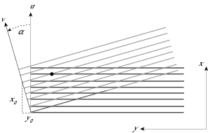
The local coordinates \( x \) and \( y \) represent the combination of two one-dimensional measurements (two dimensional, if also the constraint due to the position of the SCT module is counted) from two different sensor surfaces. The calculation of the error matrix of a SCT_SpacePoint is therefore not straightforward, especially the correlation between \( x \) and \( y \) has to be taken into account. The figure shows an idealised case in which two sensor surfaces cross each other with an angle \( \alpha \) which is around 40mrad in the SCT geometry. One sensor gives a measurement in the local coordinate \( u \) , the other in the local coordinate \( v \) . The local coordinates \( x \) and \( y \) refer to the orientation of the first sensor. With the given orientation this leads to the identity \( x=u \) . As shown in the figure, \( y \) is related to \( u \) and \( v \) via

\( u = x_0 + ( y + y_0 ) \tan\alpha \)

with

\( x_0 = v \cos\alpha \)

and

\( y_0 = v \sin\alpha \) .

From this \( y \) is found to be

\( y = u \cot\alpha - ( \cot\alpha \cos\alpha + \sin\alpha ) v \)

Therefore \( (u,v) \) transforms to \( (x,y) \) via

\( \left(\begin{array}{c} x \\ y \end{array}\right) = T \left(\begin{array}{c} u \\ v \end{array}\right) \)

with

\( T = \left(\begin{array}{cc} 1 & 0 \\ a & b \end{array}\right) \) .

where \( a \) and \( b \) are given by

\( a = \cot\alpha \simeq 25.0 \)

\( b = -(\cot\alpha \cos\alpha + \sin\alpha) \simeq -25.0 \)

From this the covariance matrix of \( x \) and \( y \) is calculated via

\( C_{x,y} = T C_{u,v} T^t \)

with

\( C_{u,v} = \left(\begin{array}{cc} \Delta u^2 & 0 \\ 0 & \Delta v^2 \end{array}\right) \) .

This results in the error matrix

\( C_{x,y} = \left(\begin{array}{cc} \Delta u^2 & a \Delta u^2 \\ a \Delta u^2 & a^2\Delta u^2 + b^2\Delta v^2 \end{array}\right) \) .

With \( \Delta u = \Delta v \) and inserting \( a \) and \( b \) this can be simplified to

\( C_{x,y} = \left(\begin{array}{cc} 1 & 25 \\ 25 & 1250 \end{array}\right) \Delta u^2 \) .

With \( \Delta u = 20\mu m\) this yields \( \Delta y = 707\mu m \). This value is slightly below the value of \( 800 \mu m\), which is realistically expected due to the ideal assumptions made in this derivation. In order to maintain the proper errors in \( x \) and \( y \), the bottom right entry of \( C_{x,y} \) is adjusted to 1600, while the rest of the matrix is kept.